Supplementary material description

This page contains additional details about the experimental setup and results discussed in the paper Data Pipeline Selection and Optimization submitted for the 21st International Workshop On Design, Optimization, Languages and Analytical Processing of Big Data (DOLAP 2019) collocated with EDBT/ICDT joint conference.

Table of Content:

1. Experiments short description
2. Experiment 1: SMBO for DPSO
   1. Detailed experimental protocol
   2. Measures and analysis
   3. Results
3. Experiment 2: Algorithm-specific Configuration
   1. Detailed experimental protocol
   2. Measures and analysis
   3. Results
   4. NMAD Calculation

Experiments short description

The paper contains two experiments:

1. Study of Sequential Model Based Optimizatoin (SMBO) to the Data Pipeline Selection and Optimization.
2. Study of if an optimal pipeline configuration is specific to an algorithm or general to the dataset.

Experiment 1: SMBO for DPSO

Detailed experimental protocol

• Datasets: Breast, Iris, Wine.
• Methods: SVM, Random Forest, Neural Network, Decision Tree.
• Dataset split: 60% for training set, 40% for test set.
• Pipeline configuration space size: 4750 configurations.

For each dataset, there is a baseline pipeline consisting in not doing any preprocessing.

Step 1

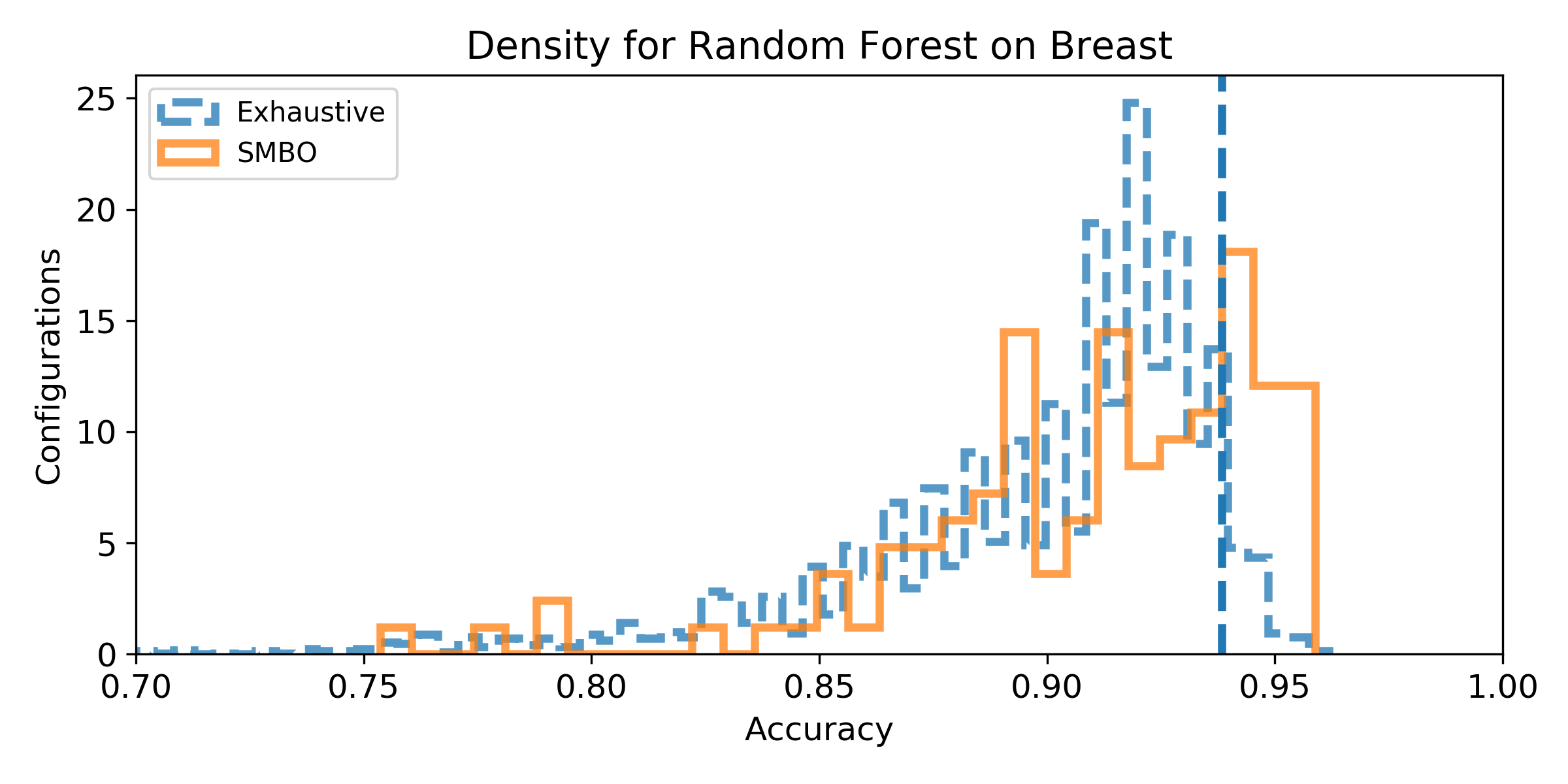
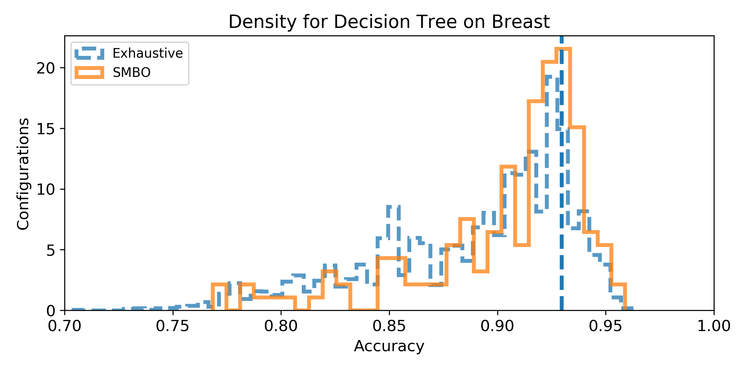
For each dataset and method, we performed an exhaustive search on the configuration space defined in details right after. For each of the 4750 configurations, a 10-fold cross-validation has been performed and the score measure is the accuracy.

Step 2

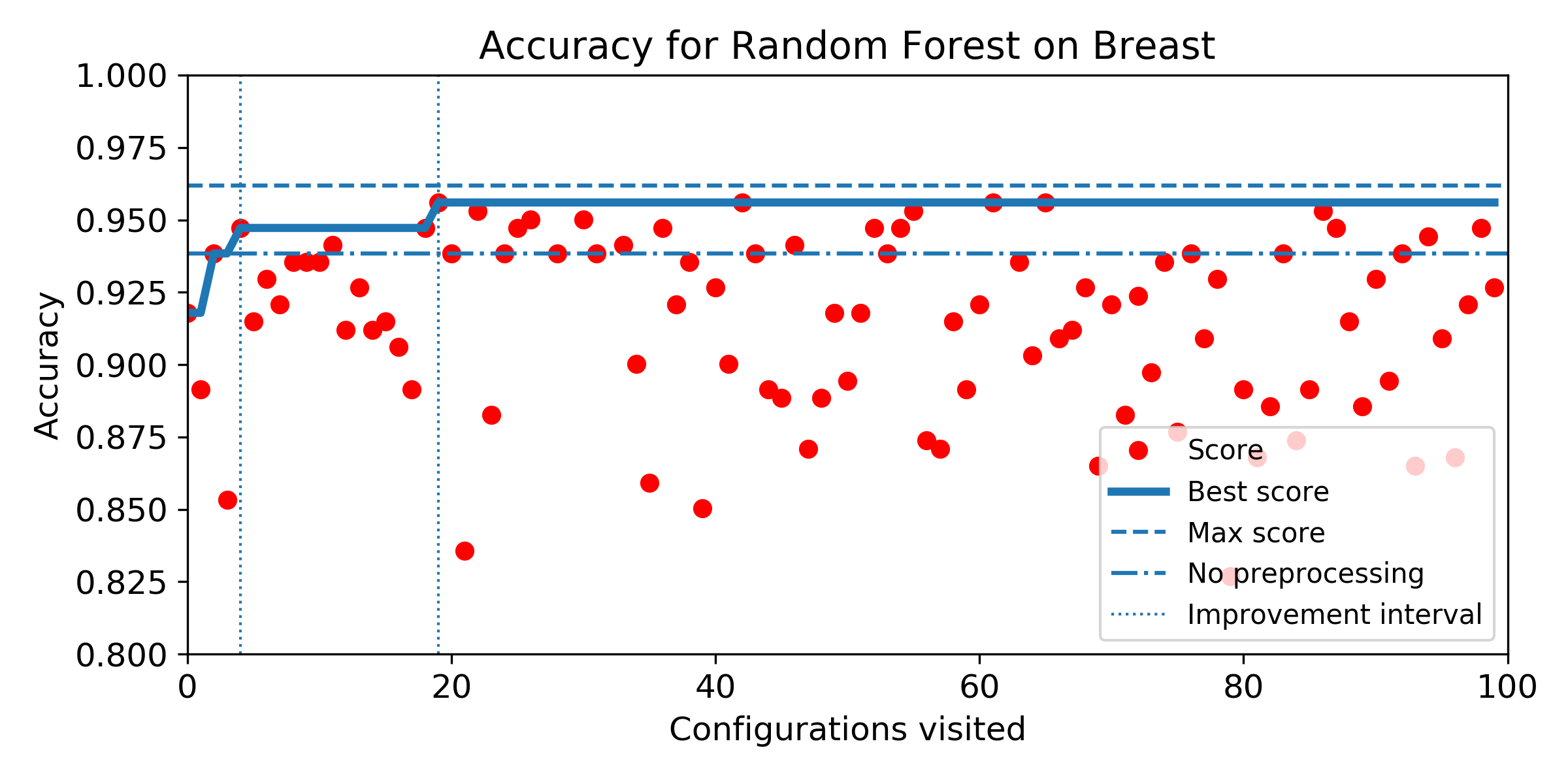
For each dataset and method, we performed a search using Sequential Model-Based Optimization (implementation provided by hyperopt) and a budget of 100 configurations to visit (about 2% of the whole configuration space). As for Step 1., we measure the accuracy obtained over a 10-fold cross-validation.

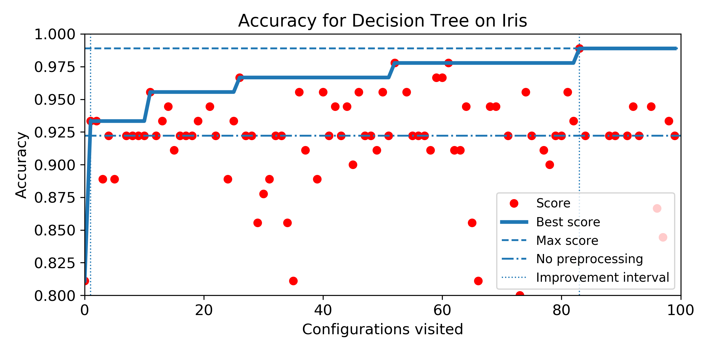
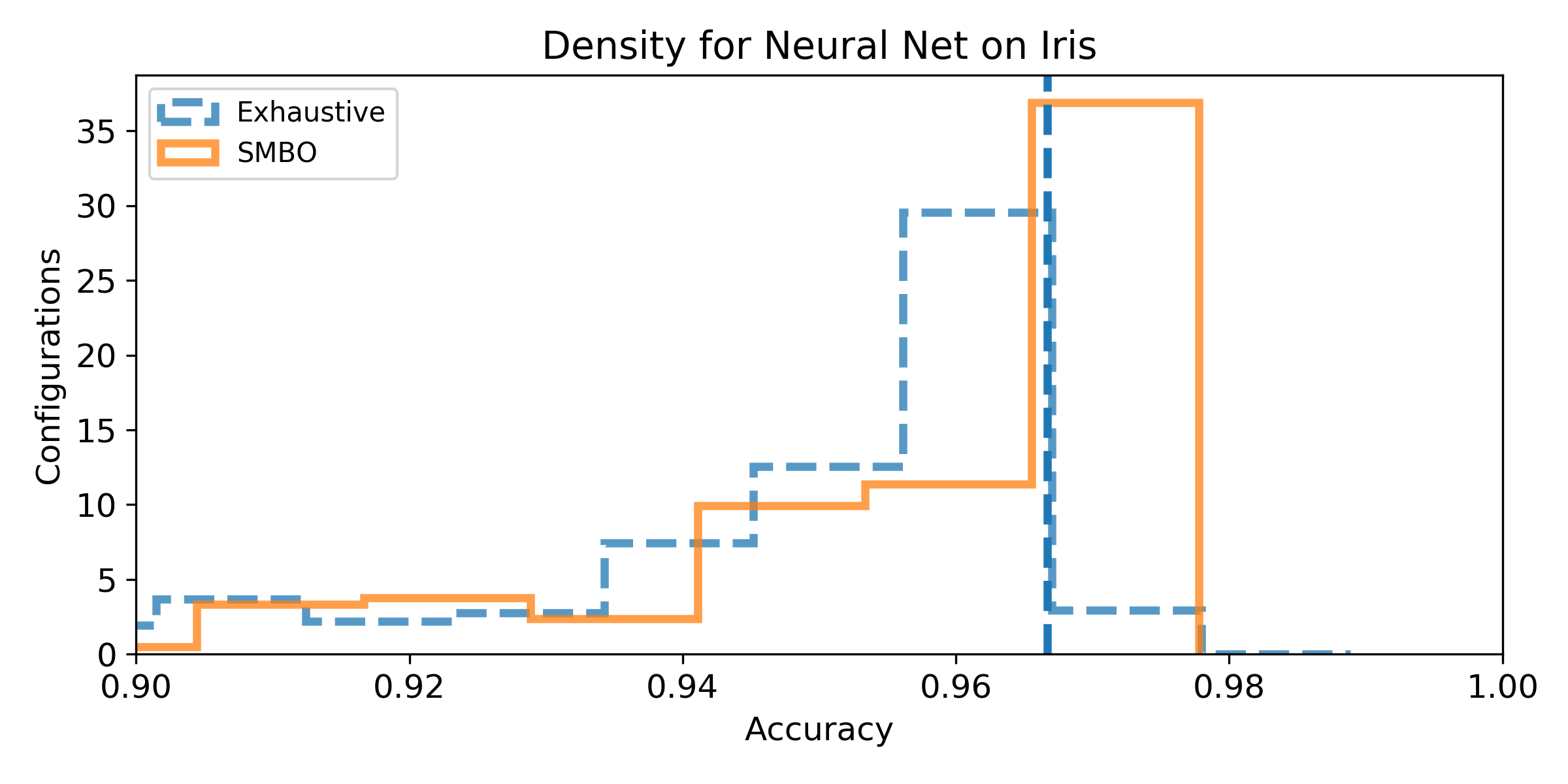
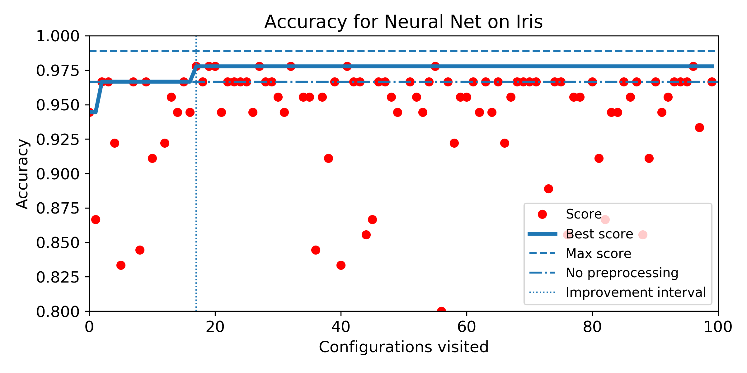
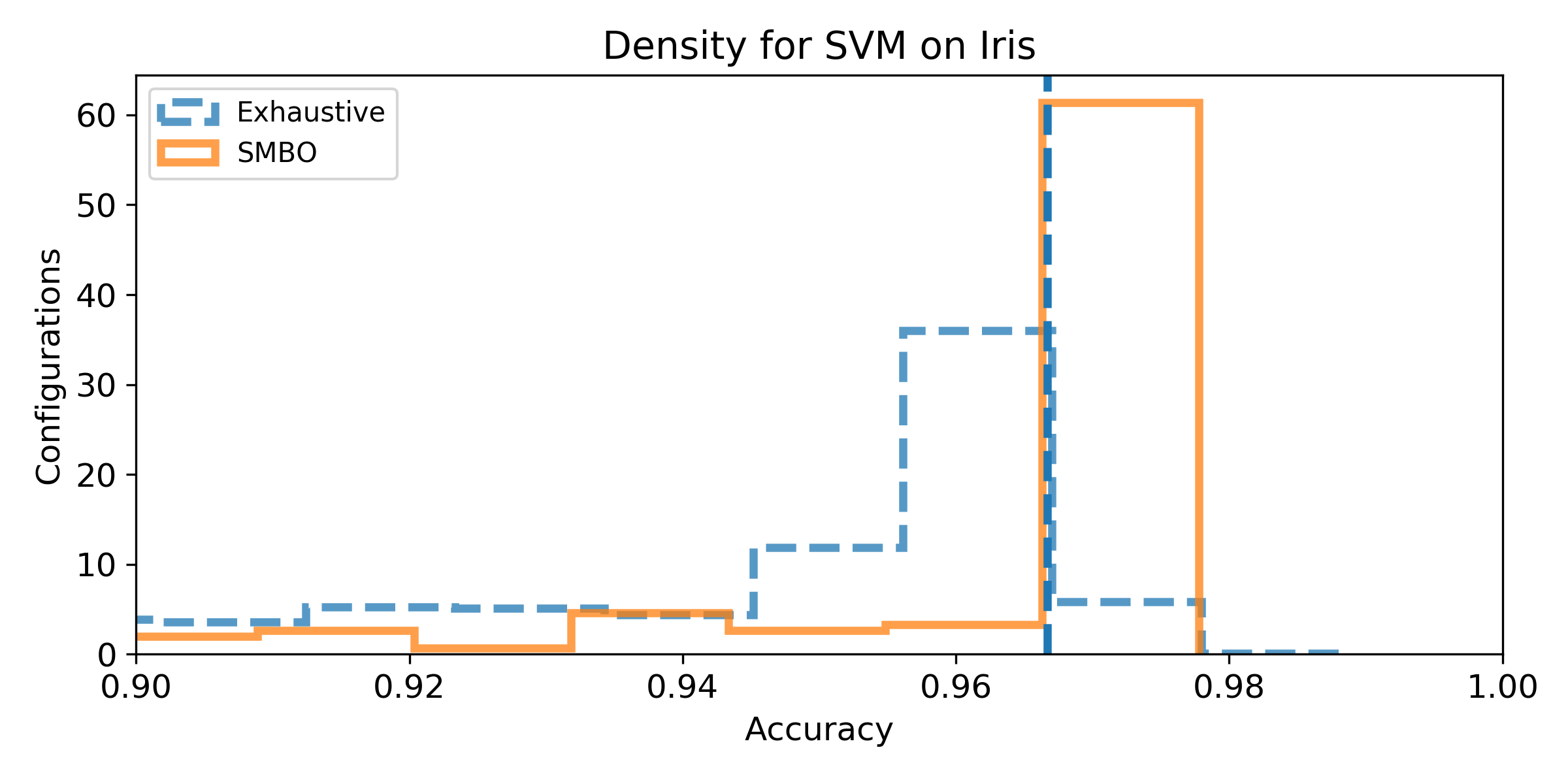
Measures and analysis

We want:

• (Q1) to quantify the achievable improvement compared to the baseline pipeline.
• (Q2) to measure how likely it is to improve the baseline score according to the configuration space.
• (Q3) to determine if SMBO is capable to improving the baseline score.
• (Q4) to measure how much SMBO is likely to improve the baseline score with a restricted budget.
• (Q5) to measure how fast SMBO is likely to improve the baseline score with a restricted budget.

To answer those questions, we generate two kind of plots:

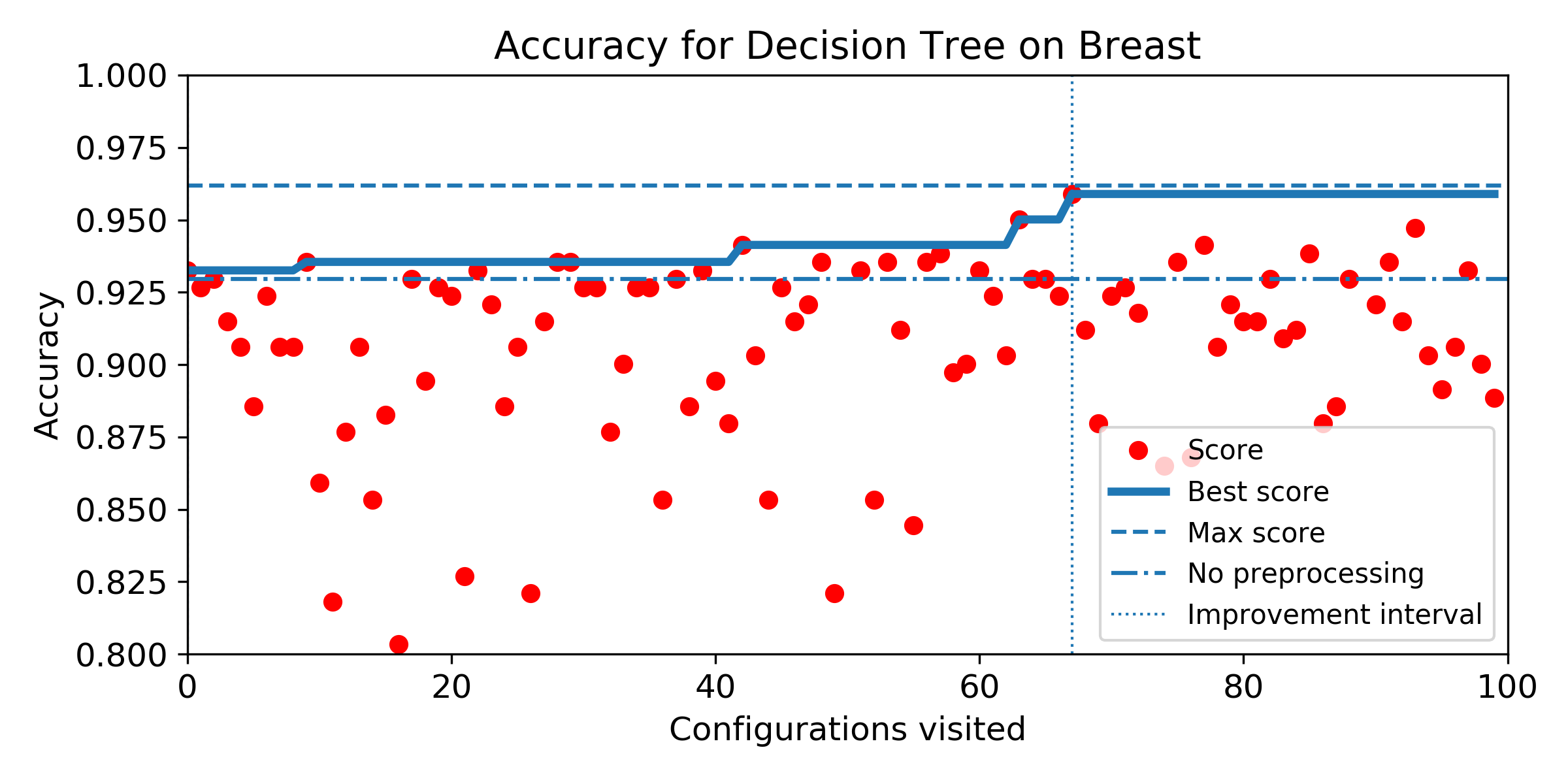
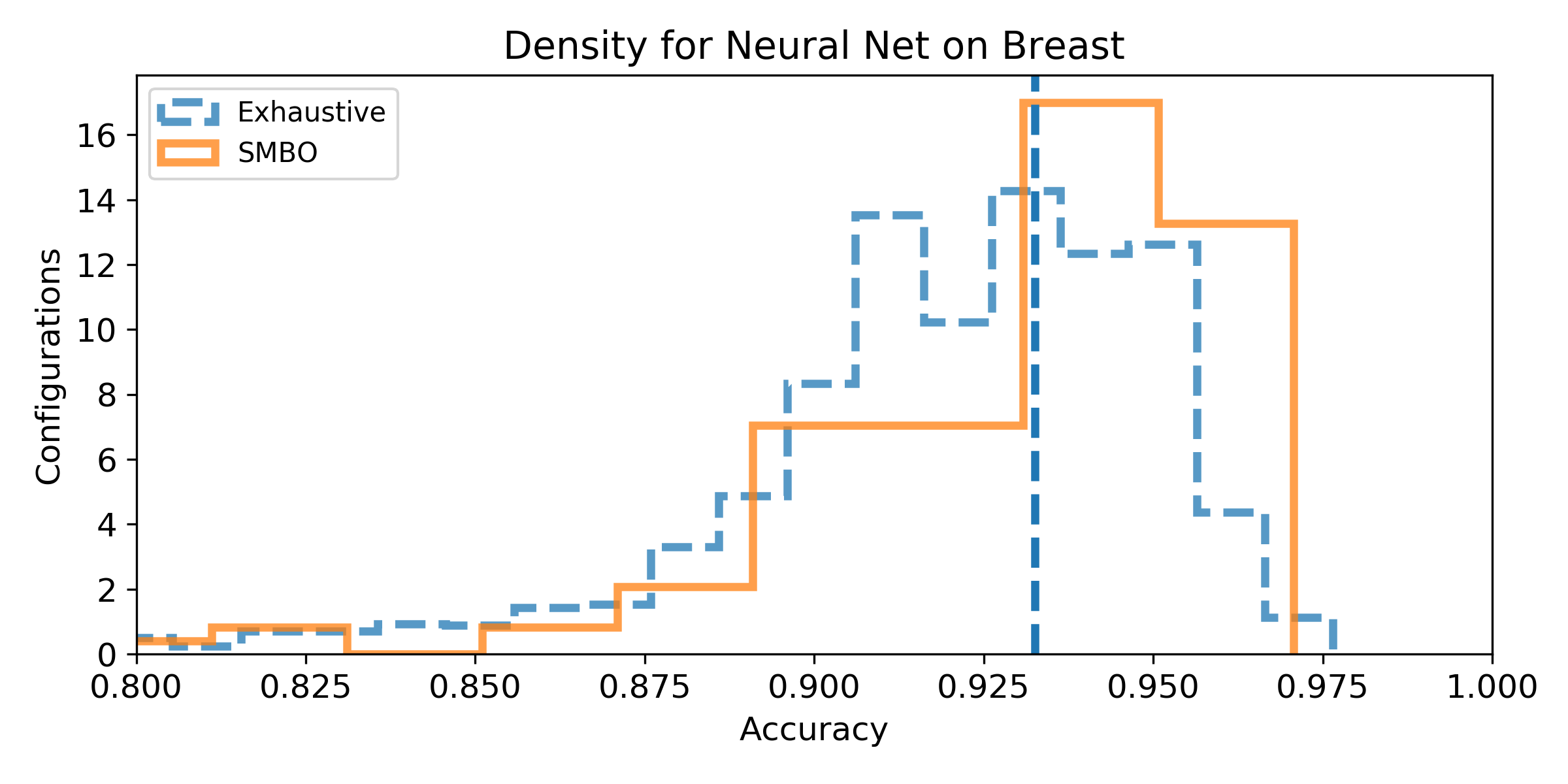
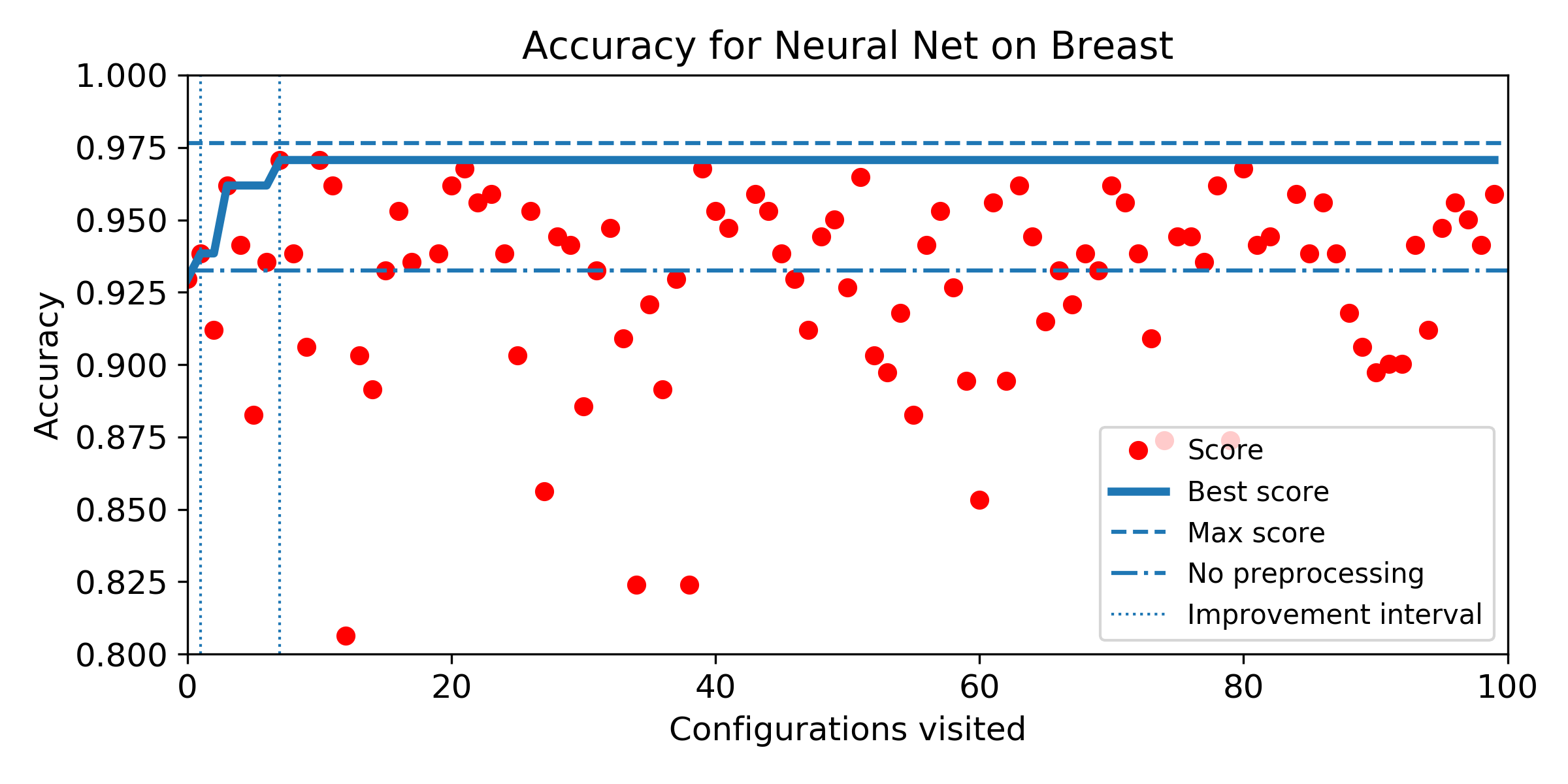
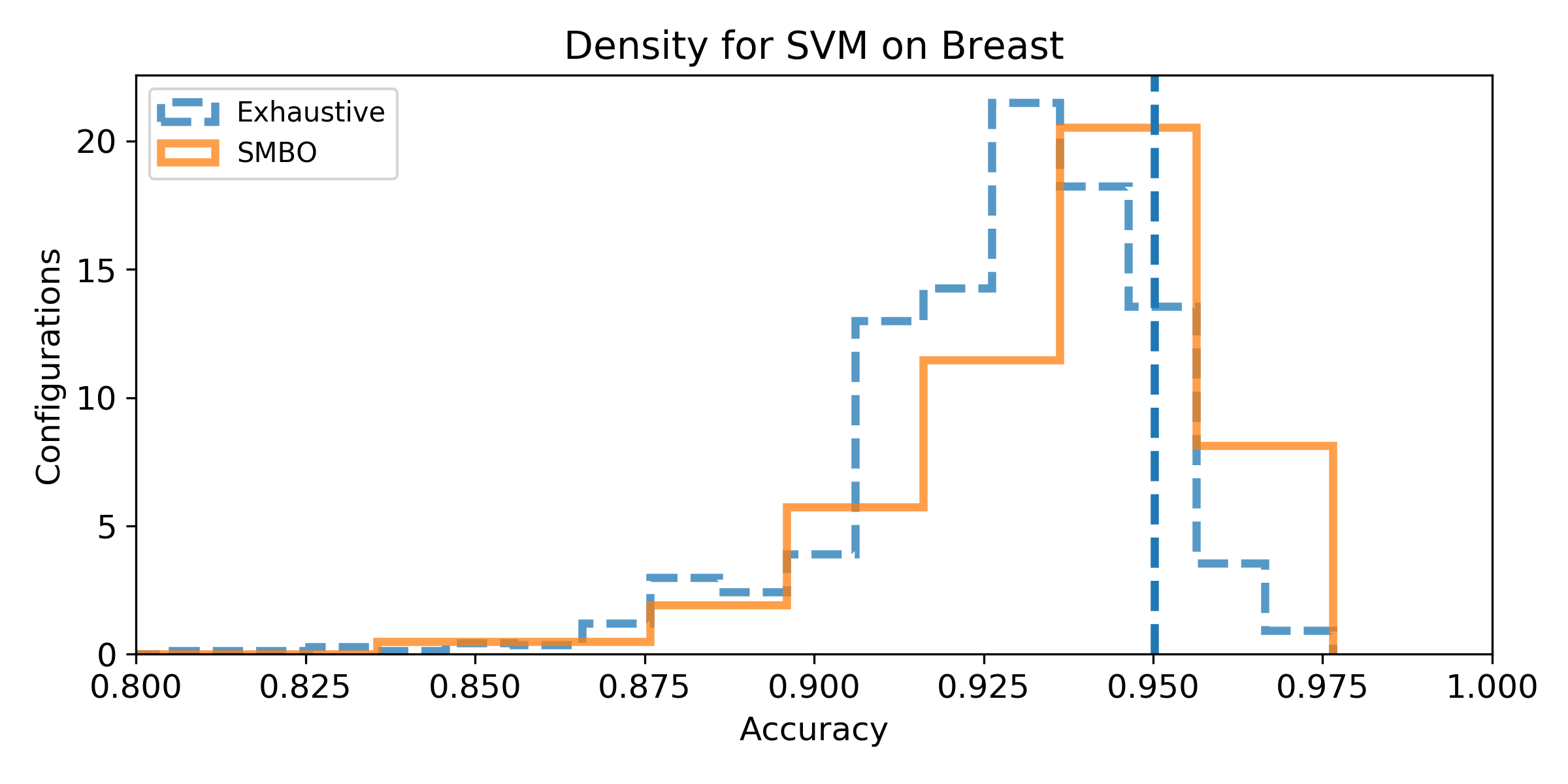
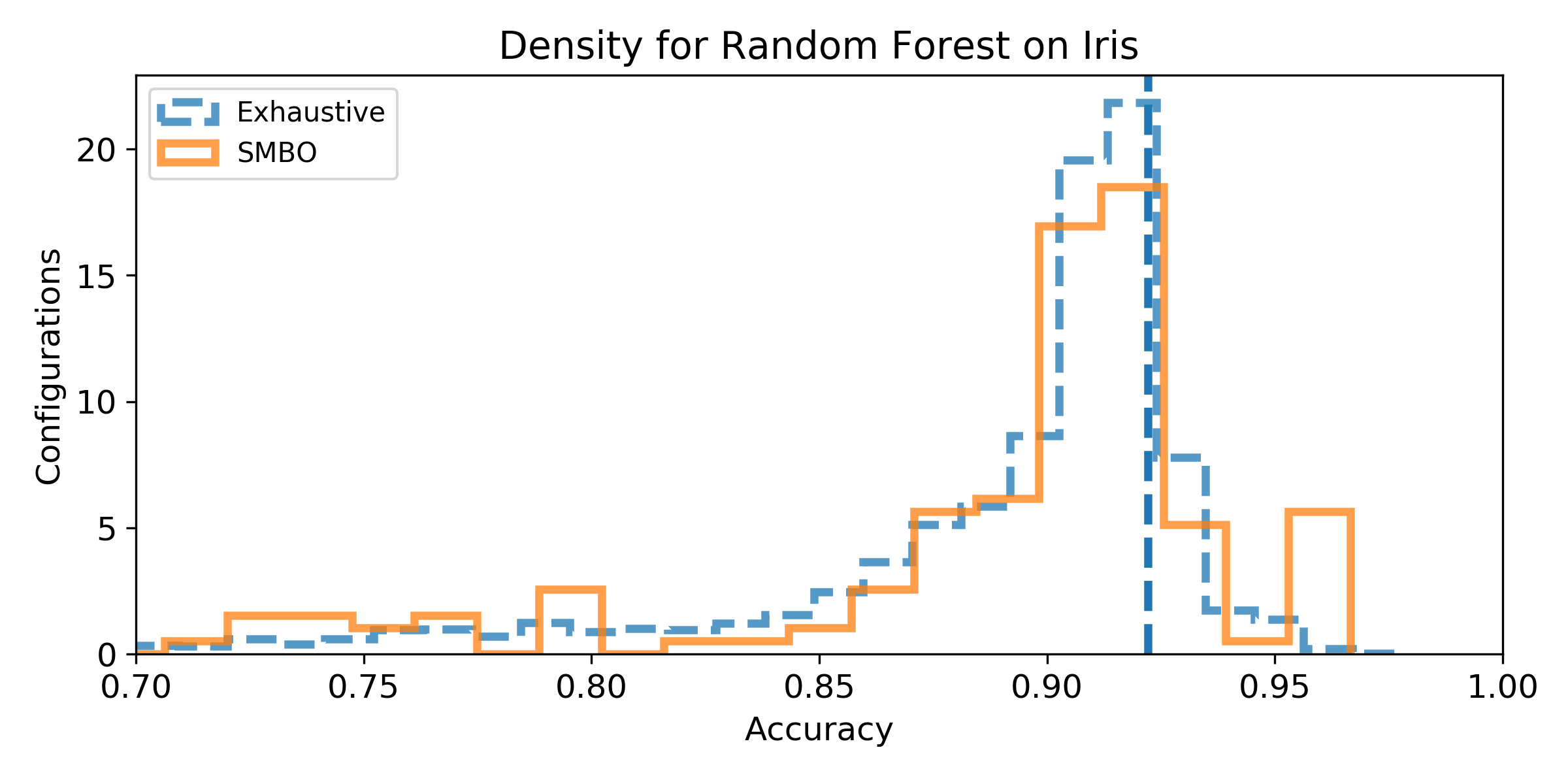
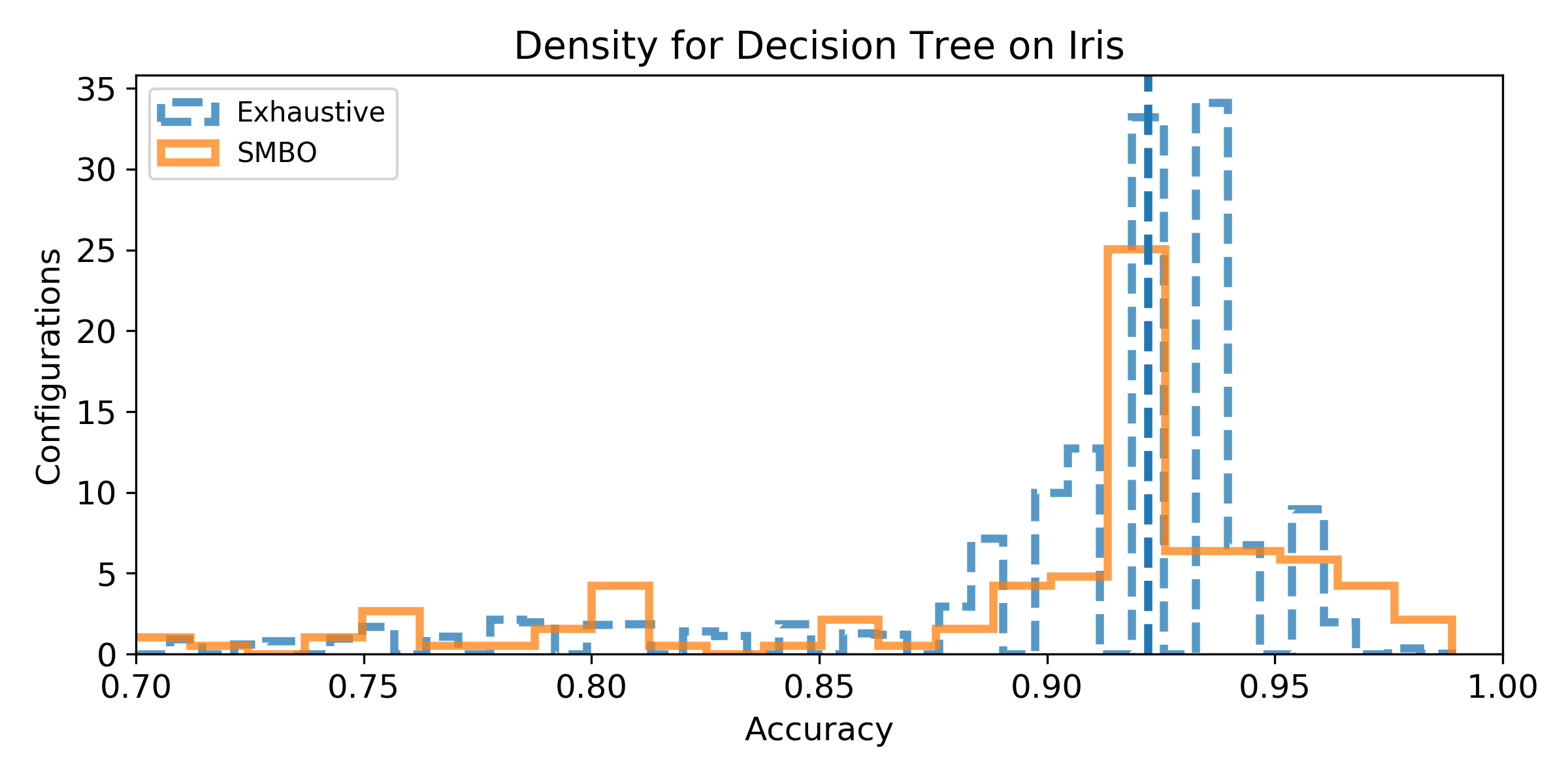
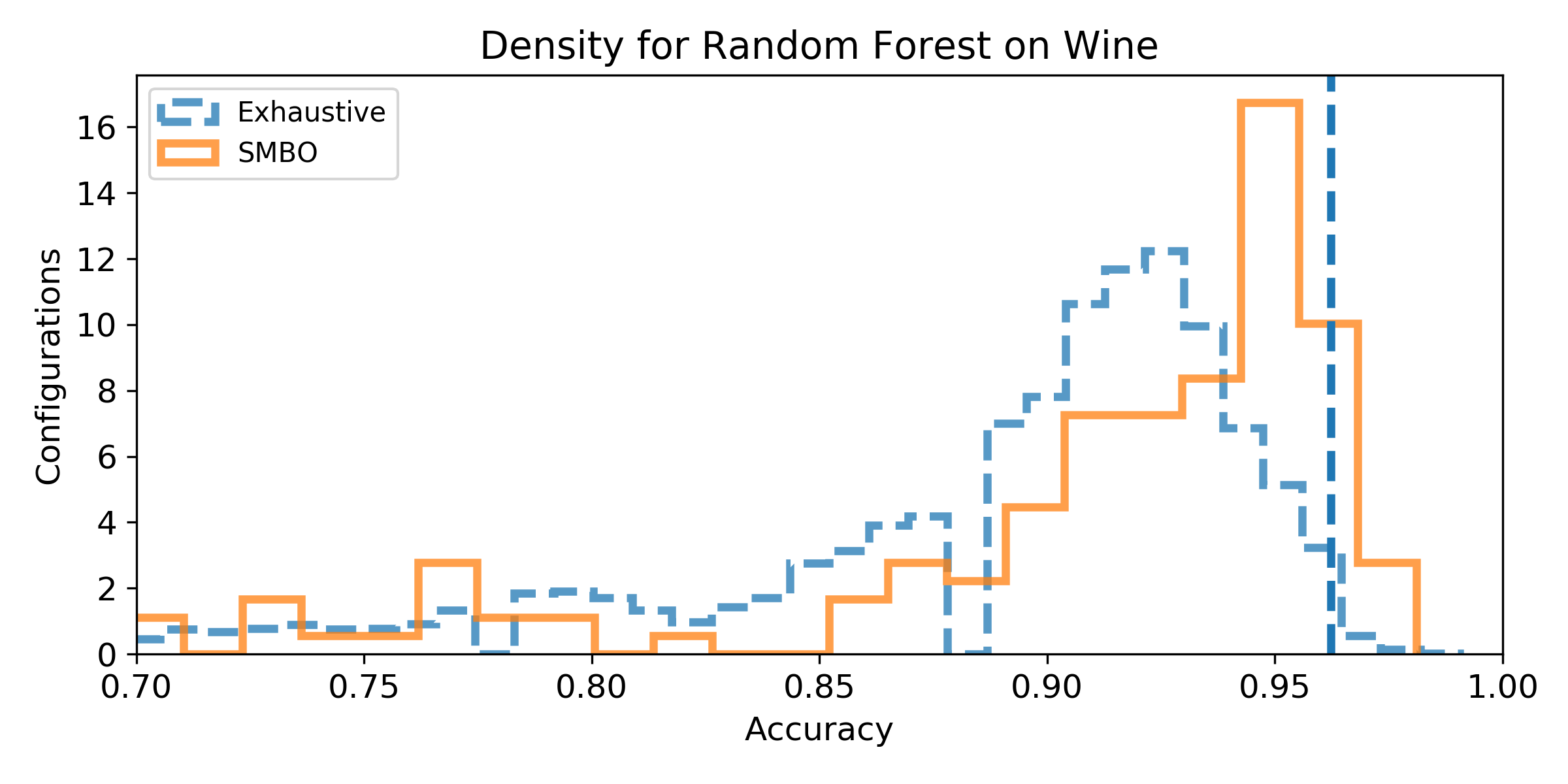
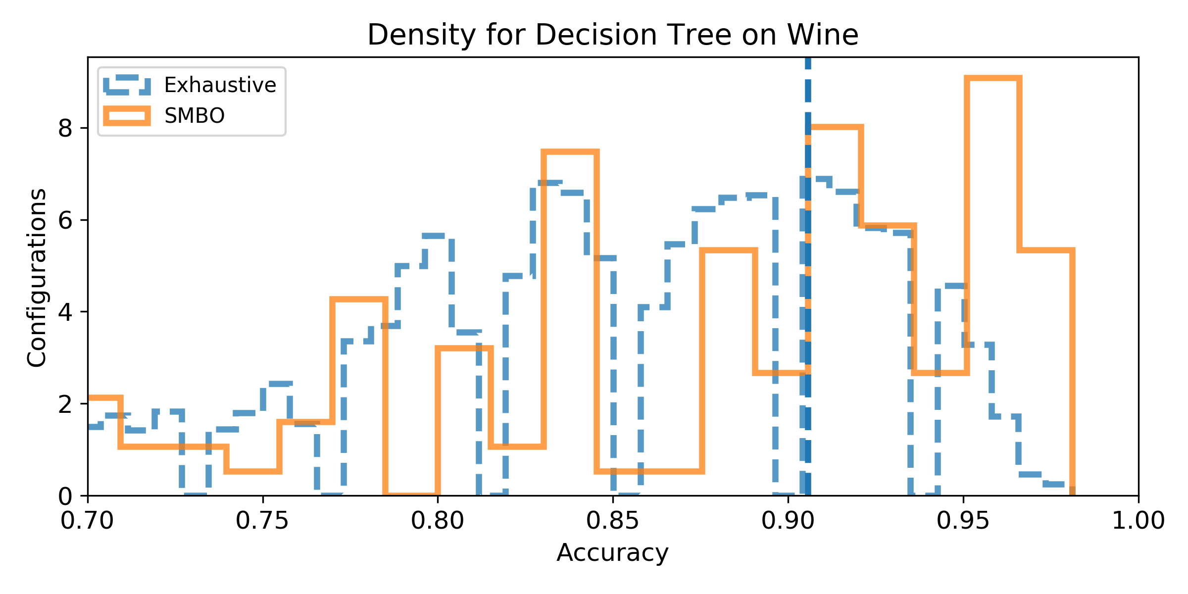
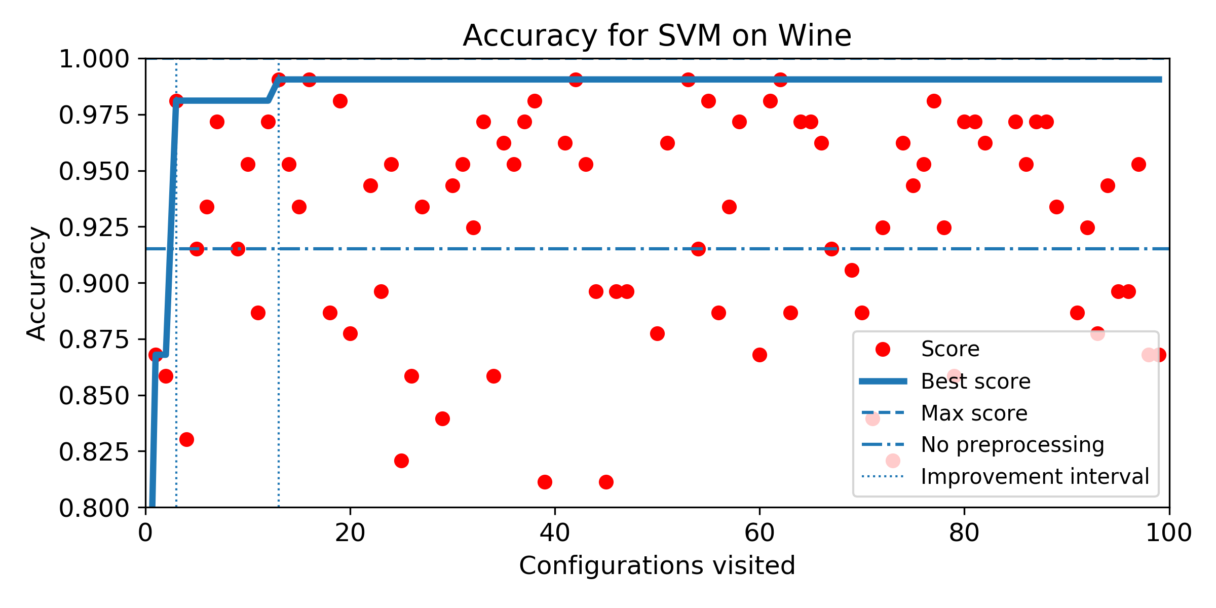
1. Density of the configuration depending on the accuracy for the exhaustive grid, and for the SMBO search. If the density is not null for accuracy higher than the baseline score, then, there exist configurations that improve the baseline score (answer to Q1). We can observe the probability to improve the baseline score (and quantify how much) by observing the proportion of the area after the baseline score vertical marker (answer to Q2). Similarely, if the density for SMBO has some support higher than the baseline score, it means SMBO search could improve (answer to Q3). If the area above the baseline score vertical marker is larger for SMBO than for the exhaustive search, then SMBO is more likely to improve the baseline than an exhaustive search (answer to Q4).
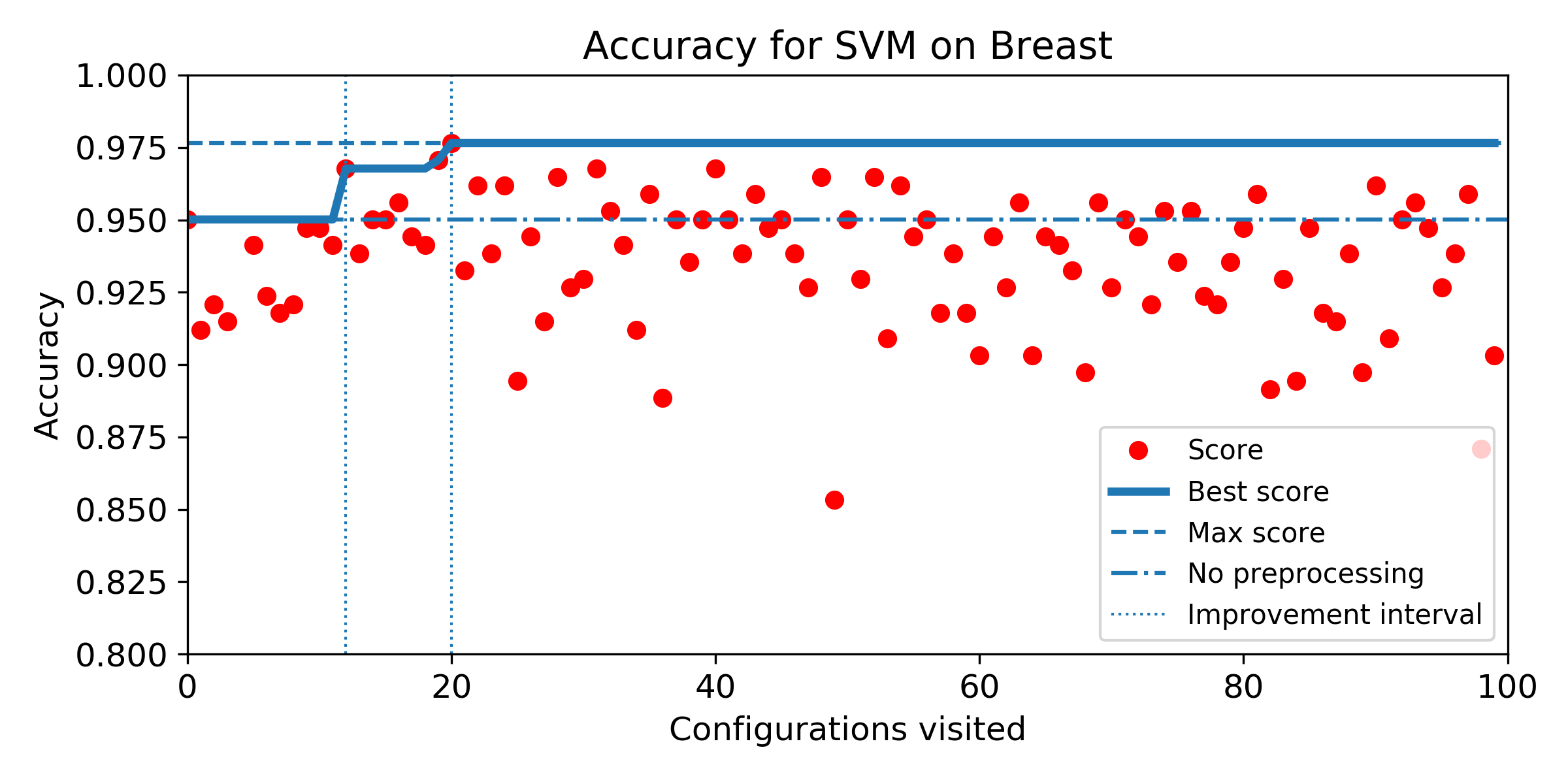
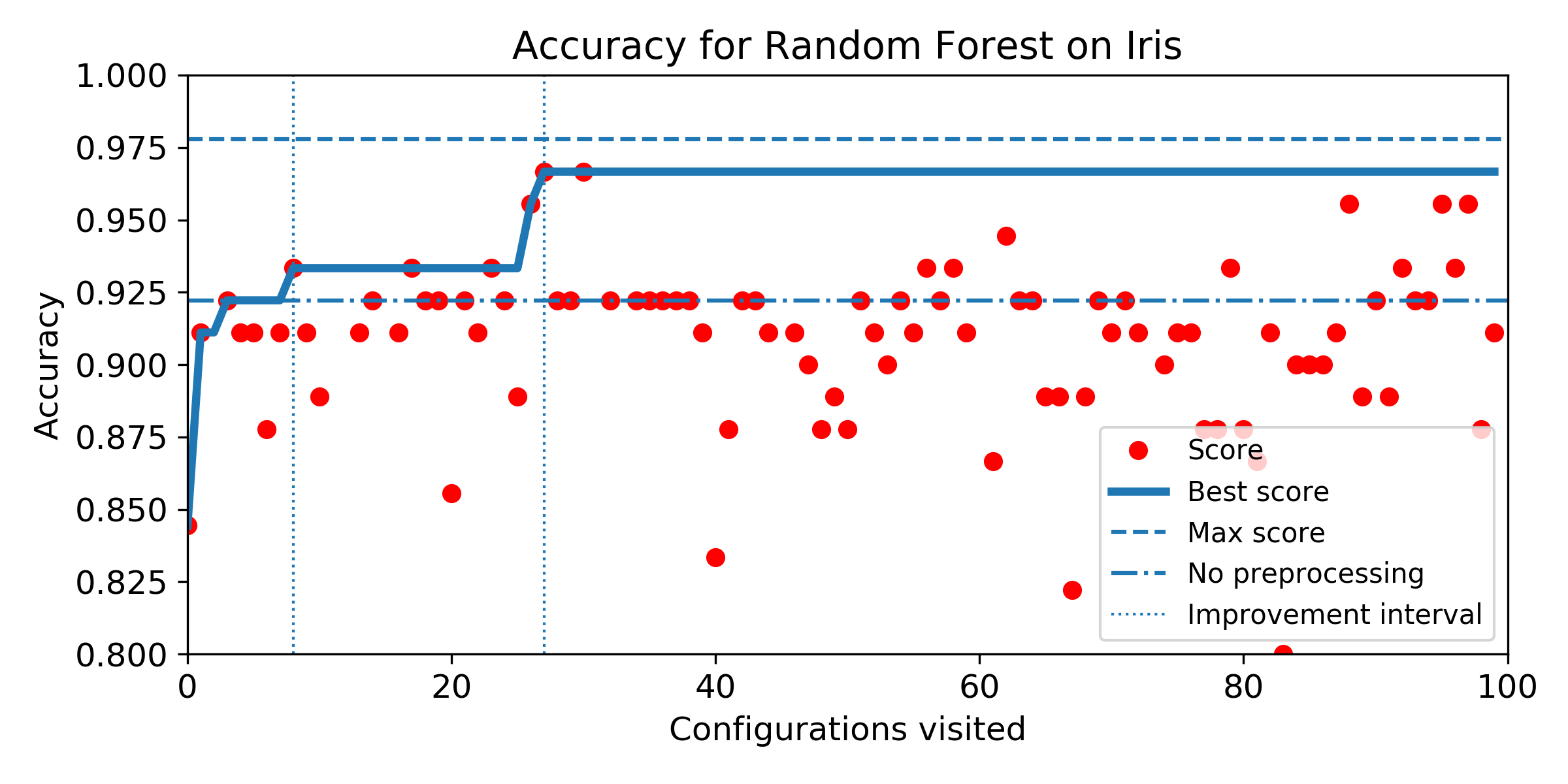
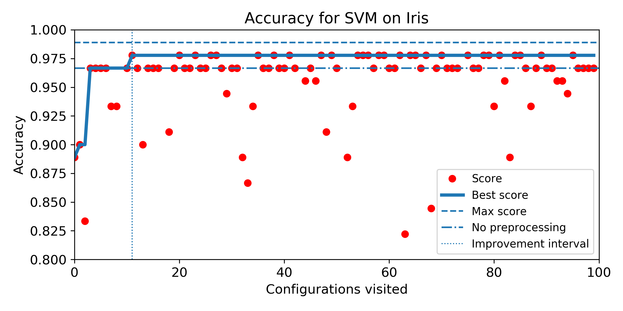
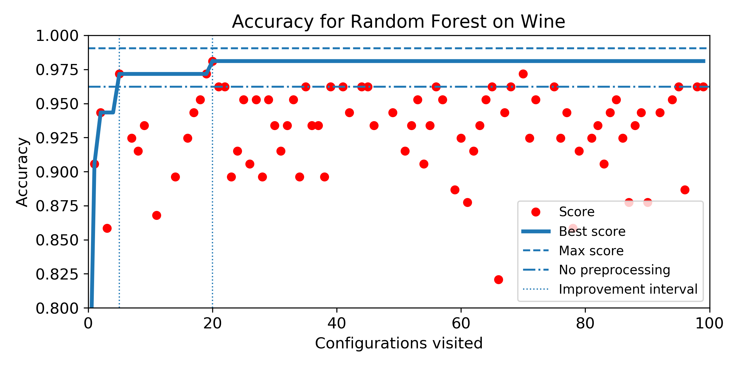
2. Evolution of score obtained configuration after configuration for SMBO search. The improvement interval is comprised between the baseline score and the best score obtained by the exhaustive search. To answer Q5, we plot horizontally the improvement interval, and plot the best score obtained iteration after iteration. SMBO improved the baseline as soon as the best score enters the improvement interval. To help visualization, we plot veritically the number of configurations needed to enter the interval and the number of configurations to visit before reaching the best score obtained over the budget of 100 configurations. For both market, the lower the better.

Pipeline prototype and configuration

The configuration space for the pipeline is composed of three operations. For each operations there are 4, 5 and 4 possible operators. Each operator has between 0 and 3 specific parameter(s). For each parameter, there is between 2 and 4 possible values. The final pipeline configuration space has a total of 4750 possible configurations.

Pipeline prototype

The pipeline prototype is composed of three sequential operations:

1. rebalance: to handle imbalanced dataset with oversampling or downsampling techniques.
2. normalizer: to normalize or scale features.
3. features: to select the most important features or reduce the input vector space dimension.

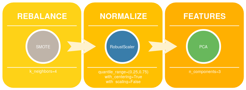
Pipeline operators

For the step rebalance, the possible methods to instanciate are:

• None: no sample modification.
• NearMiss: Undersampling using Near Miss method [1].
  Implementation: imblearn.under_sampling.NearMiss
• CondensedNearestNeighbour: Undersampling using Near Miss method [2].
  Implementation: imblearn.under_sampling.CondensedNearestNeighbour
• SMOTE: Oversampling using Synthetic Minority Over-sampling Technique [3].
  Implementation: imblearn.over_sampling.SMOTE

For the step normalizer, the possible methods to instanciate are:

• None: no normalization.
• StandardScaler: Standardize features by removing the mean and scaling to unit variance.
  Implementation: sklearn.preprocessing.StandardScaler
• PowerTransform: Apply a Yeo-Johnson transformation to make data more Gaussian-like.
  Implementation: sklearn.preprocessing.PowerTransformer
• MinMaxScaler: Transforms features by scaling each feature to [0,1].
  Implementation: sklearn.preprocessing.MinMaxScaler
• RobustScaler: Same as StandardScaler but remove points outside a range of percentile.
  Implementation: sklearn.preprocessing.RobustScaler

For the step features, the possible methods to instanciate are:

• None: no feature transformation.
• PCA: Keep the k main axis of a Principal Component Analysis.
  Implementation: sklearn.decomposition.PCA
• SelectKBest: Selecting the k most informative features according to ANOVA and F-score.
  Implementation: sklearn.feature_selection.SelectKBest
• PCA+SelectKBest: Union of features obtaines by PCA and SelectKBest.
  Implementation: sklearn.pipeline.FeatureUnion

REMARK: The baseline pipeline corresponds to the triple (None, None, None).

Pipeline operator specific configuration

• NearMiss:
  • n_neighbors: [1,2,3]
• CondensedNearestNeighbour:
  • n_neighbors: [1,2,3]
• SMOTE:
  • k_neighbors: [5,6,7]
• StandardScaler:
  • with_mean: [True, False]
  • with_std: [True, False]
• RobustScaler:
  • quantile_range:[(25.0, 75.0),(10.0, 90.0), (5.0, 95.0)]
  • with_centering: [True, False]
  • with_scaling: [True, False]
• PCA:
  • n_components: [1,2,3,4]
• SelectKBest:
  • k: [1,2,3,4]
• PCA+SelectKBest:
  • n_components: [1,2,3,4]
  • k:[1,2,3,4]

Results

The results are sorted by dataset.

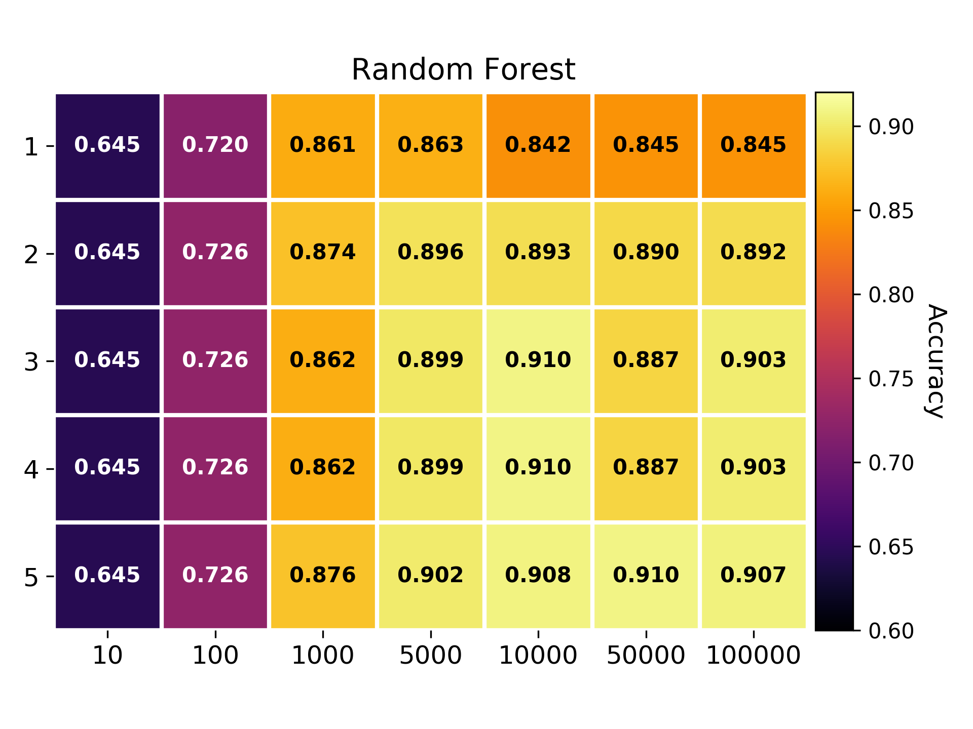
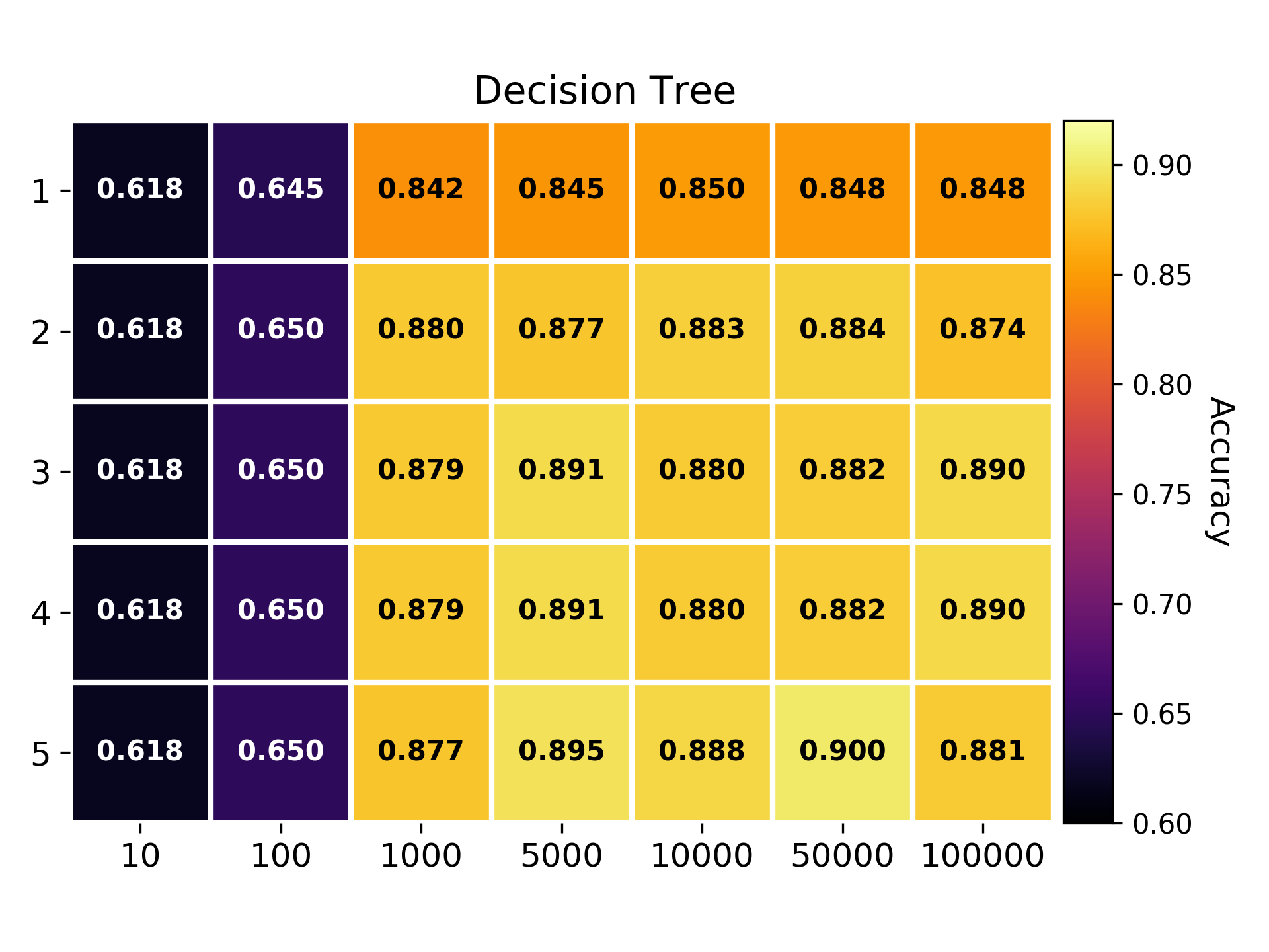
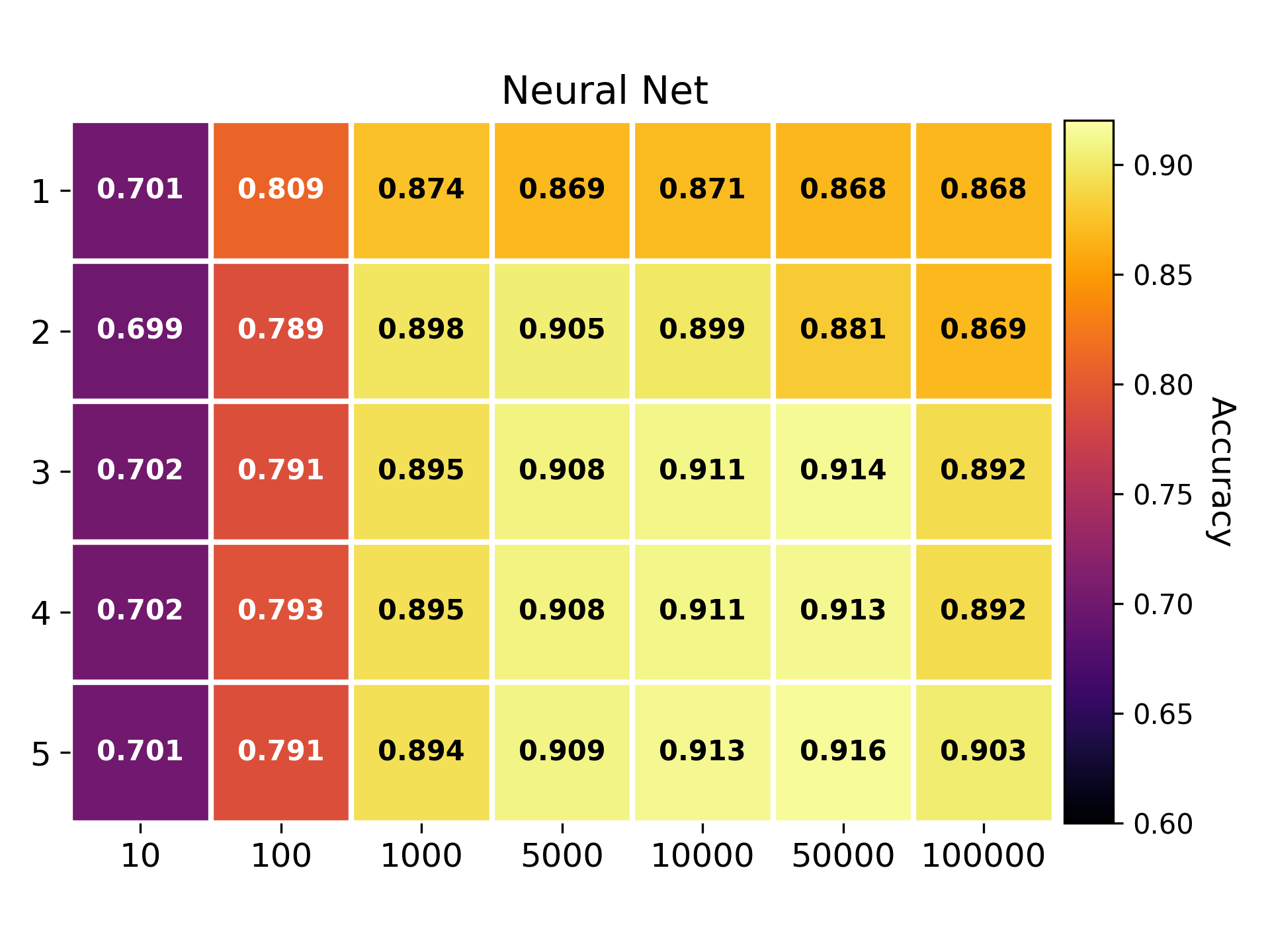
Breast dataset

Iris dataset

Wine dataset

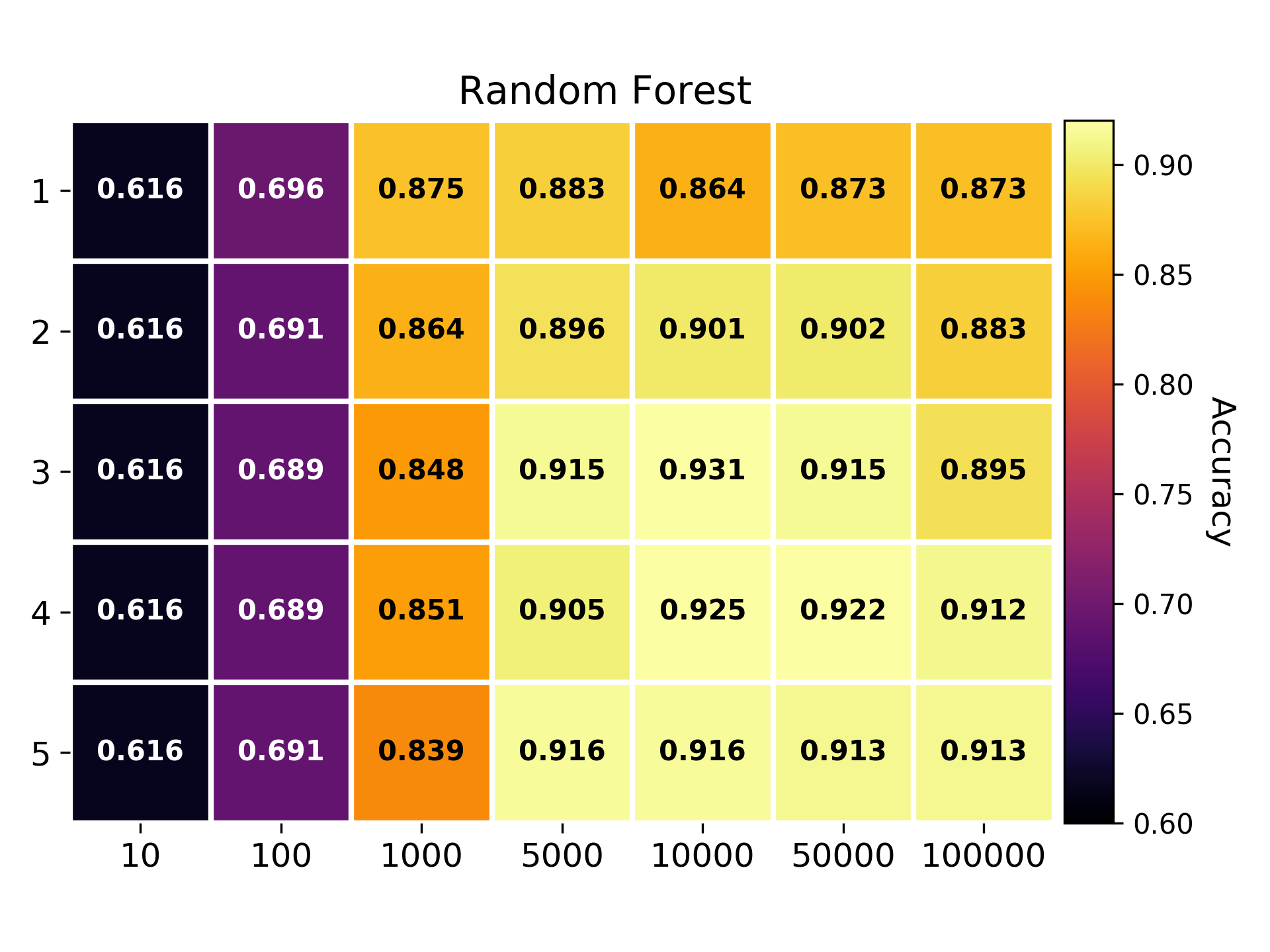
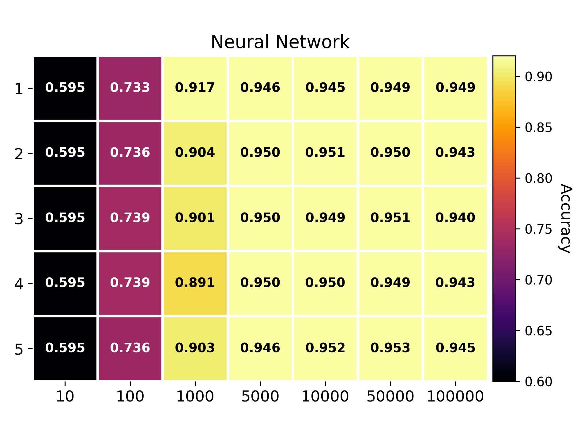
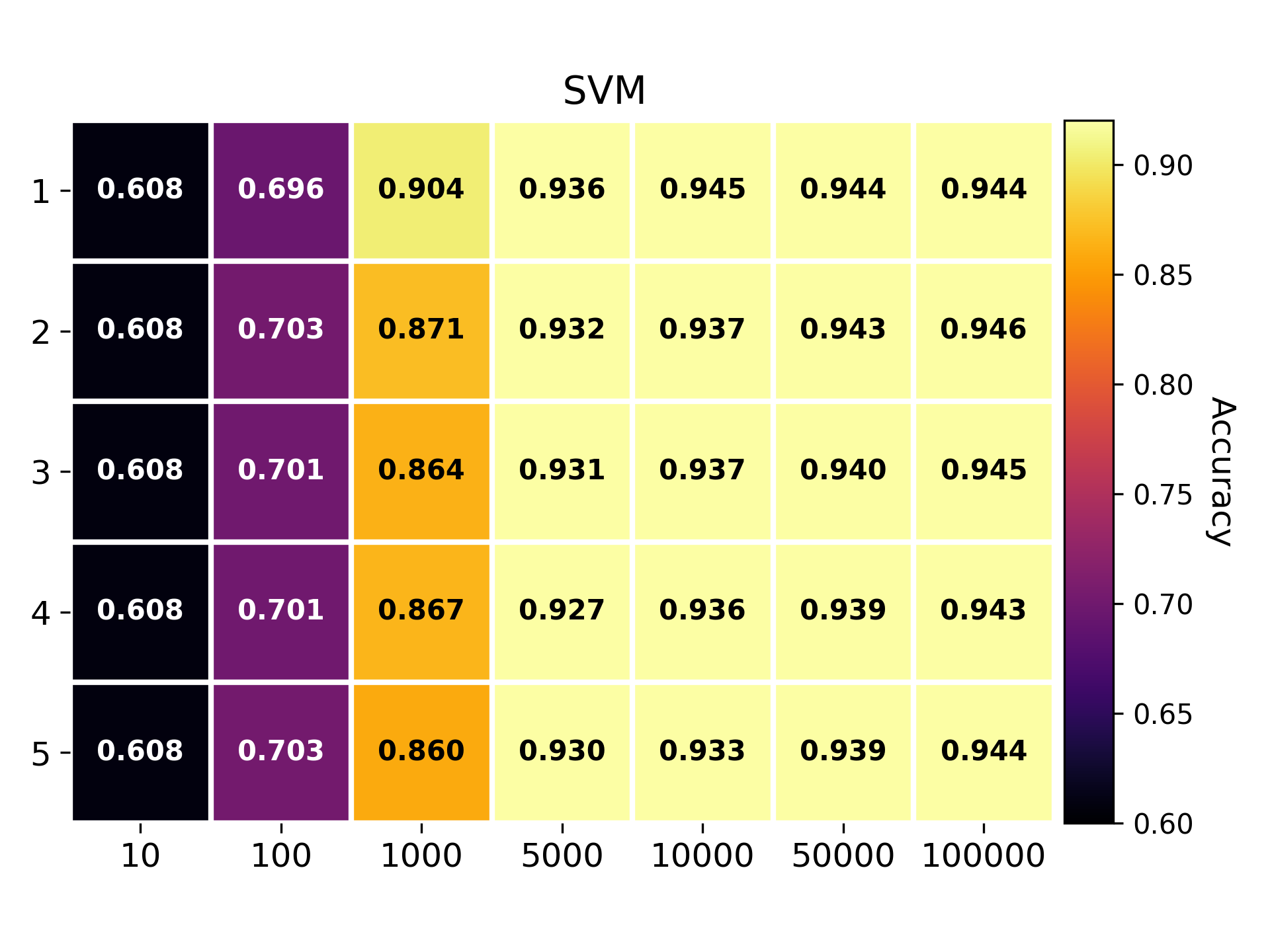
Experiment 2: Algorithm-specific Configuration

Detailed experimental protocol

• Datasets: European Court of Human Rights (1000 cases, prevalence 50\%), 20newsgroup (855 documents from the categories atheism and religion)
• Methods: SVM, Random Forest, Neural Network, Decision Tree.
• Dataset split: 60% for training set, 40% for test set.
• Pipeline configuration space size: 35 configurations.

Each document is preprocessed using a data pipeline consisting in tokenization, stopwords removal, followed by a n-gram generation. The processed documents are combined and the k top tokens across the corpus are kept to form the dictionary. Each case is turned into a Bag-of-Words using the dictionary.

There are two hyperparameters in the preprocessing phase: n the size of the n-grams, and k the number of tokens in the dictionary.

Results

The results are sorted by dataset.

ECHR dataset

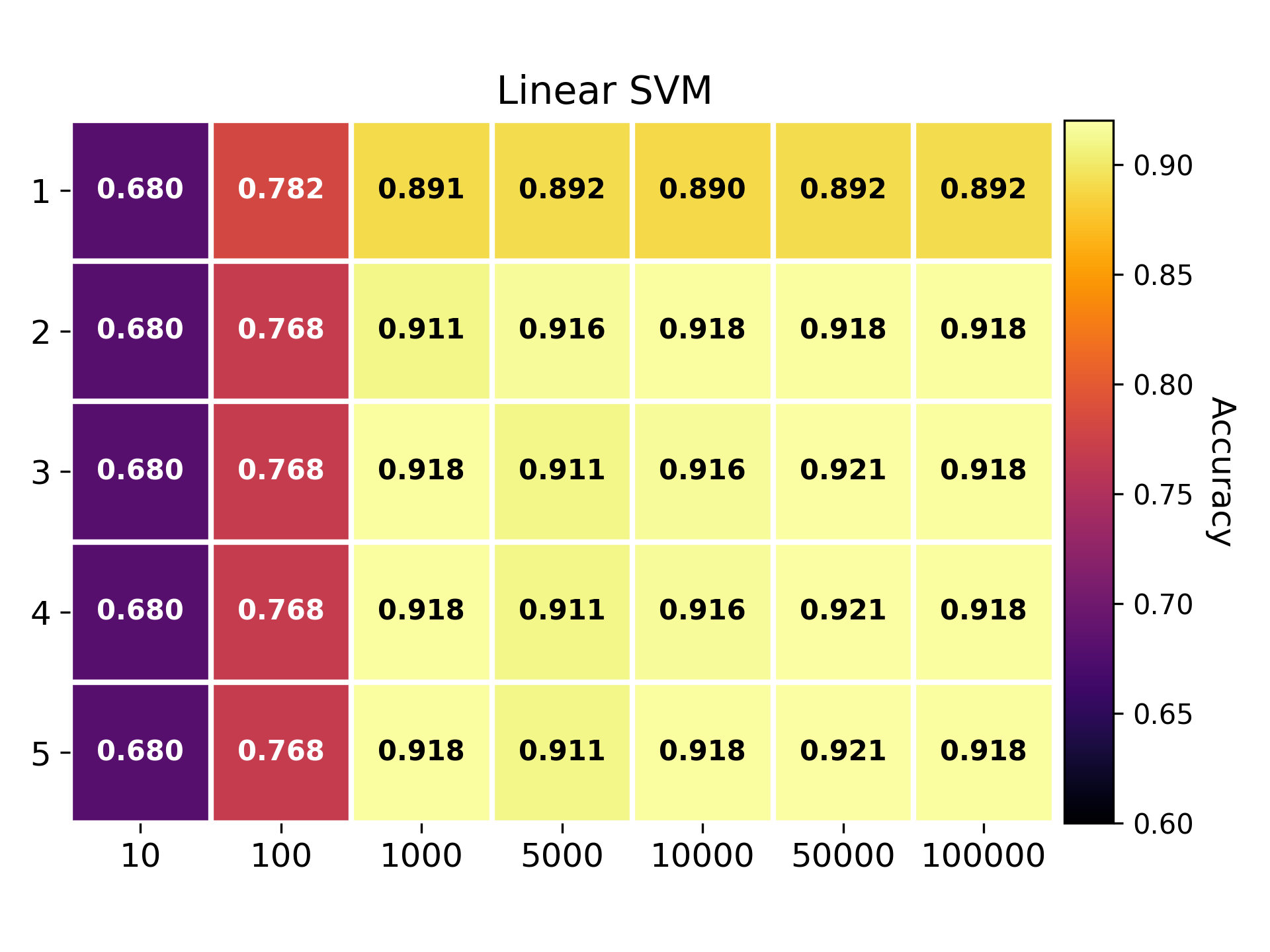
Newsgroup dataset

NMAD calculation

In this section, we provide the intermediate steps to compute the NMAD indicator. In particular, the first table display the optimal points expressed in the normalized configuration space, the second table the sample to consider for each optimal point, and the third one, the NMAD value for each optimal point.

ECHR

Method
Decision Tree
Neural Network
Random Forest	, ,
Linear SVM	, ,

Sample ECHR

Point	NMAD
	0
	0.275
	0.213
	0.175
	0.094

Newsgroup

Method
Decision Tree	,
Neural Network
Random Forest
Linear SVM

Sample Newsgroup

Point	NMAD
	0.306
	0.300
	0.356
	0.294
	0.362

References

[1] I. Mani, I. Zhang. “kNN approach to unbalanced data distributions: a case study involving information extraction,” In Proceedings of workshop on learning from imbalanced datasets, 2003.
[2] P. Hart, “The condensed nearest neighbor rule,” In Information Theory, IEEE Transactions on, vol. 14(3), pp. 515-516, 1968.
[3] N. V. Chawla, K. W. Bowyer, L. O.Hall, W. P. Kegelmeyer, “SMOTE: synthetic minority over-sampling technique,” Journal of artificial intelligence research, 321-357, 2002.